Solar Swimming Pool Heating - Thermo-Economic Analysis
To follow along with my hand written work or view the code print out, download the Thermo-Economic model here.
This analysis was performed with Engineering Equation Solver (EES), a non-linear equation solver that includes various resources for thermodynamics, heat transfer, unit handling, and economic functions.
Introduction
If you live in a sunny climate that can still be cold, like the high desert of the Rocky Mountain front range, you may have thought about adding solar panels to your home. But what about using solar energy for heat? Can a system be installed to adequately heat your swimming pool to a comfortable temperature throughout the year?
In this analysis, I investigated upgrading a traditional heated pool with solar collector as a method to reduce natural gas water heating costs.
Solar flux collectors, also commonly known as solar thermal collectors, are used for various applications, including heating swimming pools. These systems capture and convert solar energy into heat energy, which is then transferred to a fluid (usually water or a glycol mixture) circulating through the collector. This heated fluid can then be used to heat water in a swimming pool, reducing the dependency on conventional energy sources such as natural gas or electricity.
You can read more about how they work, here.
Baseline System
The unmodified heated pool system consists of the swimming pool itself, a water pump, and a natural gas powered water heater.
A schematic of the baseline system is shown below in Figure 1.

Known Parameters - Baseline
Several parameters are known about the system. The pool water is modeled as an imcompressible fluid and the system is assessed during steady state operation.
| Variable | Value | Comment |
|---|---|---|
| Q_dot_pool | 9.5 [kW] | Pool Heat Loss Rate |
| v_w | 0.001 [m^3/kg] | Pool Water Specific Volume |
| C_w | 4200 [J/kg-K] | Pool Water Specific Heat Capacity |
| T_pool | 80 [F] | Pool Water Setpoint Temperature |
| T_o | 70 [F] | Ambient Temperature |
| P_o | 14.7 [psia] | Ambient Pressure |
| eta_h | 0.95 [-] | Natural Gas Heater Efficiency |
| T_f | 1200 [F] | Natural Gas Combustion Temperature |
| ngc | 1.25 [$/therm] | Natural Gas Cost |
| eta_p | 0.4 [-] | Water Pump Efficiency |
| ec | 0.12 [$/kW-hr] | Electricity Cost |
The pump curve of the system is defined via the following equations.
EQ 1. ∆P = ∆P_dh*(1-(Vol_dot/Vol_dot_oc))
EQ 2. ∆P_dh = 150 [Pa-min/rev]*N [rev/min]
EQ 3. Vol_dot_oc = 5x10^-7 [m^3-min/s-rev]*N [rev/min]
EQ 4. ∆P_h = 3x10^12 [Pa-s/m^6]*Vol_dot^2
States & Balances - Baseline
State [4-1] - Pool
Mass Balance
In = Out —> m_dot[1] = m_dot[4] = m_dot
During steady state operaiton, the mass flowrate of water into the pool equals the mass flowrate of water leaving the pool.
Energy Balance
m_dot * h[4] = Q_dot_pool + m_dot * h[1]
The energy associated with the mass of the water entering and leaving the system is related to the enthalpy of the water, which is defined by the properties of the water.
Entropy Balance
S_dot_gen_pool = (Q_dot_pool / T_pool) + m_dot * (s[4]-s[1])
Entropy generation inside the pool can be calculated to measure exergy destruction.
State [1] - Pump Inlet
State Properties
T[1] = T_pool = 80 [F]
P[1] = P_o = 14.7 [psi] (Assumption for P[2] == Ambient)
Pump inlet water properties are equal to the properties of the water leaving the pool.
Incompressible Fluid Model
u[1] = c_w * T[1]
h[1] = c_w * T[1] - v_w * P[1]
State [1-2] - Water Pump
Mass Balance
m_dot_2 = m_dot_1 = m_dot = Vol_dot/v_w
Water mass flow rate during steady state operation can also be calculated from the volumetric flowrate of the water, divided by the specific volume of the water (determined by T and P).
Energy Balance
m_dot[1] * h[1] + W_dot_p = m_dot[2] * h[2]
Energy from the pump is added to the water from state 1 to 2.
Entropy Balance
m_dot[1] * s[1] + S_dot_gen_p = m_dot[2] * s[2]
(s[2]-s[1]) = c_w * ln(T[2]/T[1])
Reversible Energy Balance
m_dot[1] * h[1] + W_dot_p_s = m_dot[2] * h_s[2]
h_s[2] = c_w * T[1] + v_w * P[2]
Pump Performance Balance
eta_p = 0.4 = W_dot_p_s / W_dot_p
The water pump is marked with a 40% efficiency compared to a perfectly reversible pump with no entropy generation.
State [2] - Pump Outlet
P[2] = P[1] + ∆P
T[2] = From E-bal, State 1-2
State fixed with Pressure and Temperature
State [2-3] - Piping
P[3] = P[2] (Ignoring pressure loss through pipe resistance / geometry)
T[3] = T[2]
Mass Balance
m_dot[3] = m_dot[2]
Energy Balance
m_dot[3]*h[3] = m_dot[2]*h[2]
State [3] - Water Heater Inlet
T[3] = T[2]
P[3] = P[2]
h[3] = h[2]
u[3] = u[2]
State fixed with Pressure and Temperature
State [3-4] - Water Heater
Energy Balance
m_dot[3] * h[3] + Q_dot_f = m_dot[4]*h[4]
h[4] = c_w * T[4] + v_w * P[4]
Entropy Balance
m_dot[3] * s[3] + (Q_dot_f/T_f) + S_dot_gen,h = m_dot[4] * s[4]
S_dot_gen,h = m_dot(s[4]-s[3]) - Q_dot_f/T_f
(s[4]-s[3]) = c_w * ln(T[4]/T[3])
Heat Exchanger Efficiency
eta_h = 0.95 = Q_dot_f,s / Q_dot_f
Reversible Energy Balance
m_dot[3] * h[3] + Q_dot_f,s = m_dot[4] * h_s[4]
h_s[4] = c_w * T[3] + v * P[4]
State [4] - Heater Outlet
P[4] = P[3] - ∆P_h
∆P_h = 3E12 [Pa-s/m^6] * Vol_dot^2
u[4] = c_w * T[4]
h[4] = solved from Reversible Energy Balance and Heat Exchanger Efficiency
Performance Calculations - Baseline
Pump Curves - Baseline

System Curves - Baseline

Performance Metrics - Baseline

Economic Calculations - Baseline

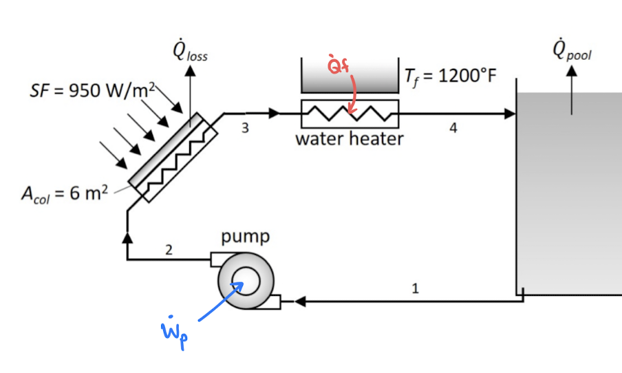
Solar Modified System

Known Parameters - Modified
| Variable | Value | Comment |
|---|---|---|
| SF | 950 [W/m^2] | Solar Flux |
| A_col | 6 [m^2] | Solar Collector Surface Area |
| ∆P_col | 5E12 [(Pa-s^2/m^6)*Vol_dot^2] | Pool Water Specific Heat Capacity |
States & Balances - Modified
State [2-3] - Solar Flux Collector

State [3] - Solar Collector Outlet

Performance Calculations - Modified


Economic Calculations - Modified

Economic Comparison
The baseline heating system comes with higher operational costs, driven by the inefficiencies of conventional methods. In contrast, the upgraded system introduces smarter solutions like integrating a solar collector, which offsets a significant portion of the heating load. This means less reliance on expensive energy sources and more money saved over time.
For example, the upgraded system reduces water heating costs from $0.4074/hour in the baseline to $0.2384/hour by covering 41.6% of the heating load through solar input. That’s a huge efficiency boost with direct cost savings for every hour the system is in use.
Conclusion
This comparison shows a clear advantage: upgrading the system cuts operational costs, plain and simple. By lowering the amount you’re spending on heat while still meeting the same demand, the upgraded setup pays for itself over time. If saving money is the goal, the numbers make this a no-brainer.